We can also define spaces in other ways, and then try to find cell complex structures for them. For example, the real projective n-space ${\mathbb{R}\textrm{P}^{n}}$ is defined as the space of all lines through the origin in ${\mathbb{R}^{n+1}}$. Each such line is determined by a unit vector, except that the negative of every vector is identified with the same line, so we can consider ${\mathbb{R}\textrm{P}^{n}}$ to be ${S^{n}}$ with antipodal points identified.

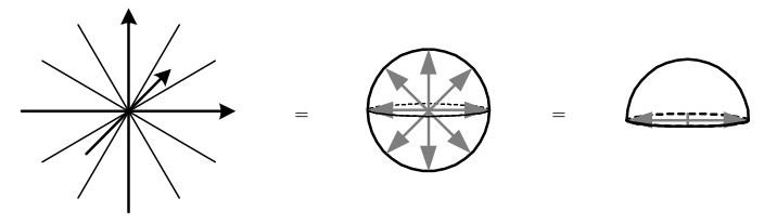
Alternatively, we can look at ${\mathbb{R}\textrm{P}^{n}}$ as the unit vectors in the upper hemisphere only, since the lower hemisphere is made up of all negatives of the upper; except that now, antipodal points of the boundary are identified. But the upper hemisphere is ${D^{n}}$ and its boundary is ${S^{n-1}}$ with antipodal points identified, or ${\mathbb{R}\textrm{P}^{n-1}}$. Thus ${\mathbb{R}\textrm{P}^{n}}$ is obtained by attaching an ${n}$-cell to ${\mathbb{R}\textrm{P}^{n-1}}$, and by induction we can see that ${\mathbb{R}\textrm{P}^{n}}$ has a cell complex structure with one cell in each dimension up to ${n}$.

The identifications in the above constructions of ${\mathbb{R}\textrm{P}^{2}}$ are not easily visualized, since they cannot be embedded in ${\mathbb{R}^{3}}$. In contrast, ${\mathbb{R}\textrm{P}^{1}}$, also called the real projective line, is ${D^{1}}$ with boundary ${S^{0}}$ having antipodal points identified, i.e. the line segment with the endpoints identified; in other words ${\mathbb{R}\textrm{P}^{1}\cong S^{1}}$, the circle. Another way of viewing this is to consider the map from each line (omitting the origin) to its slope, with the vertical line then being mapped to infinity, resulting in ${\mathbb{R}P^{1}\cong\mathbb{R}_{\infty}\cong S^{1}}$, where ${\mathbb{R}_{\infty}\equiv\mathbb{R}\cup\left\{ \infty\right\}}$ denotes the space ${\mathbb{R}}$ along with a point at infinity:

$$\begin{aligned}\mathbb{R}^{2} & \to\mathbb{R}P^{1}\cong\mathbb{R}_{\infty}\\ \left\{ \left(x,mx\right),m,0\neq x\in\mathbb{R}\right\} & \mapsto m\\ \left\{ \left(0,y\right),y\in\mathbb{R}\right\} & \mapsto\infty \end{aligned}$$

We can also define the complex projective n-space ${\mathbb{C}\textrm{P}^{n}}$, which is the space of all lines through the origin in ${\mathbb{C}^{n+1}}$. In this case one has a cell complex structure with one cell in each even dimension up to 2${n}$. ${\mathbb{H}\textrm{P}^{n}}$ can similarly be defined, but ${\mathbb{O}\textrm{P}^{n}}$ can only be defined for ${n<3}$ due to lack of associativity. By generalizing the reasoning above, we have ${\mathbb{C}\textrm{P}^{1}\cong\mathbb{C}_{\infty}\cong S^{2}}$; ${\mathbb{H}\textrm{P}^{1}\cong\mathbb{H}_{\infty}\cong S^{4}}$; and ${\mathbb{O}\textrm{P}^{1}\cong\mathbb{O}_{\infty}\cong S^{8}}$. As manifolds, the projective spaces are all closed, i.e. compact and without boundary.